Students
Graphing Calculator benefits students from elementary to university levels. It helps them grasp math concepts and cultivates problem solving skills.
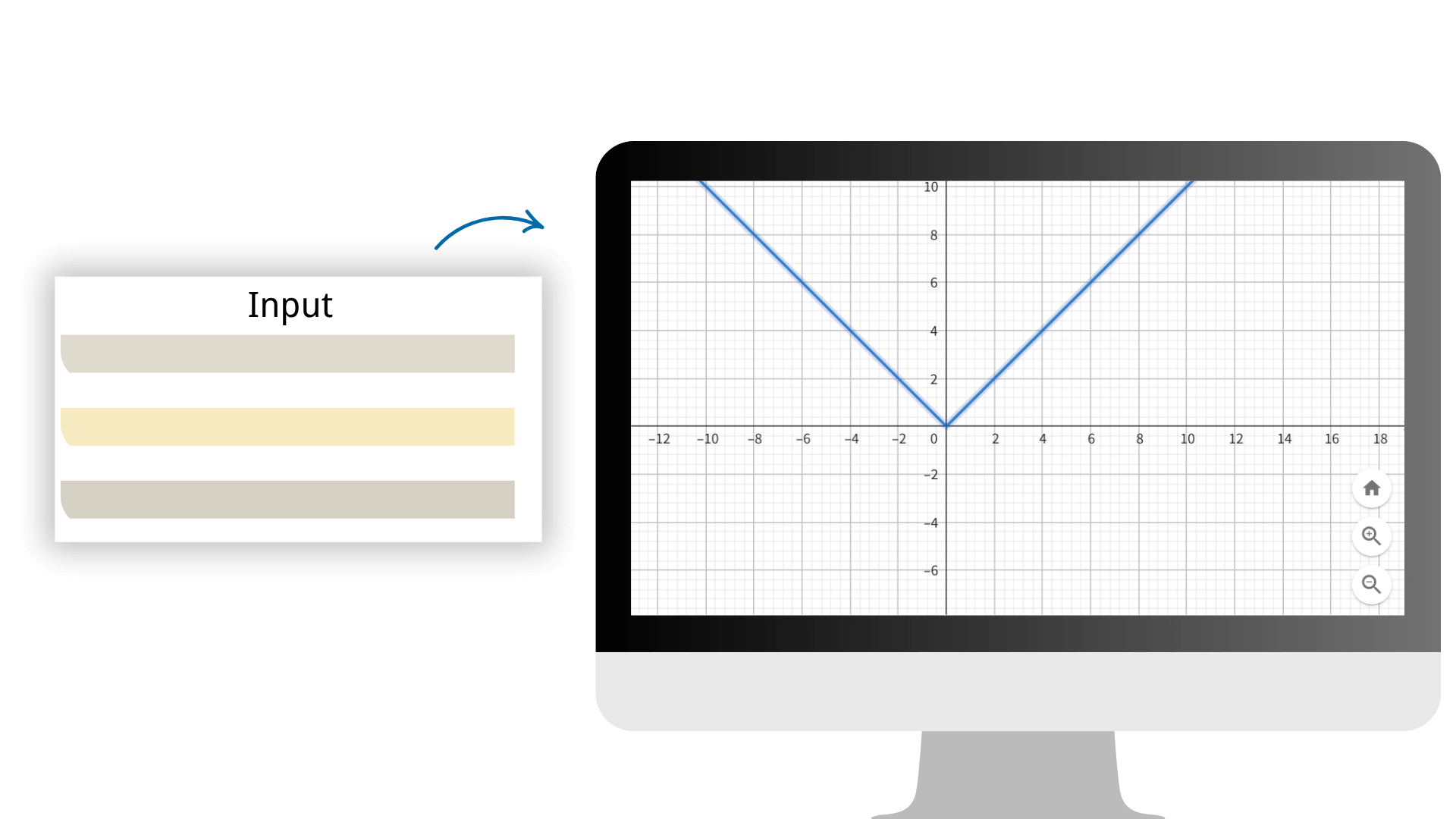
A graphing calculator can solve equations and draw graphs of functions, helping you to intuitively and accurately understand the changing patterns of functions.
Graphing Calculator is a powerful and technologically advanced drawing tool that helps us plot function graphs, perform complex calculations, and conduct data analysis. By adjusting parameters to affect the transformation of graphics, mathematical learning and research become more intuitive, efficient and interesting.
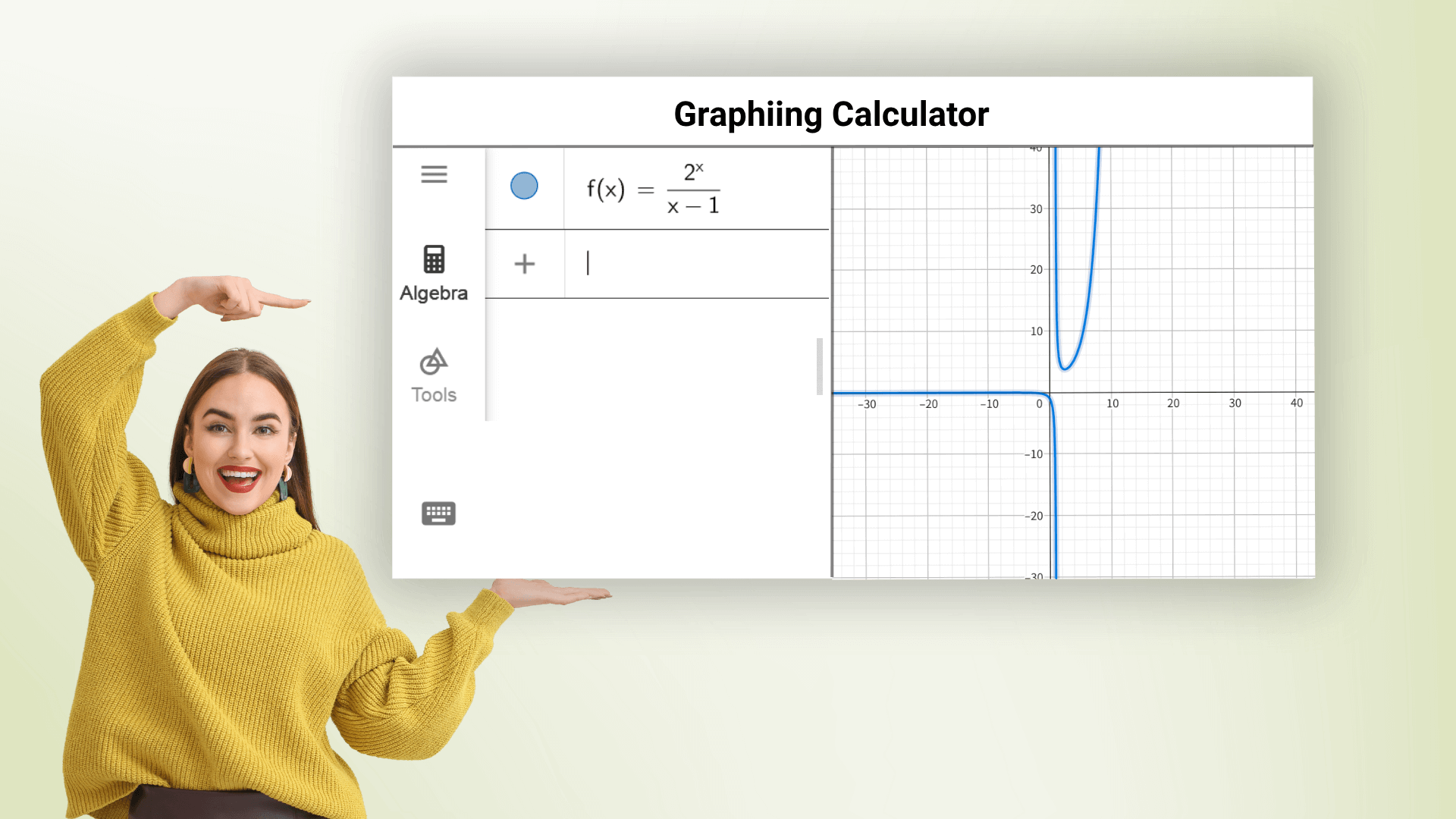
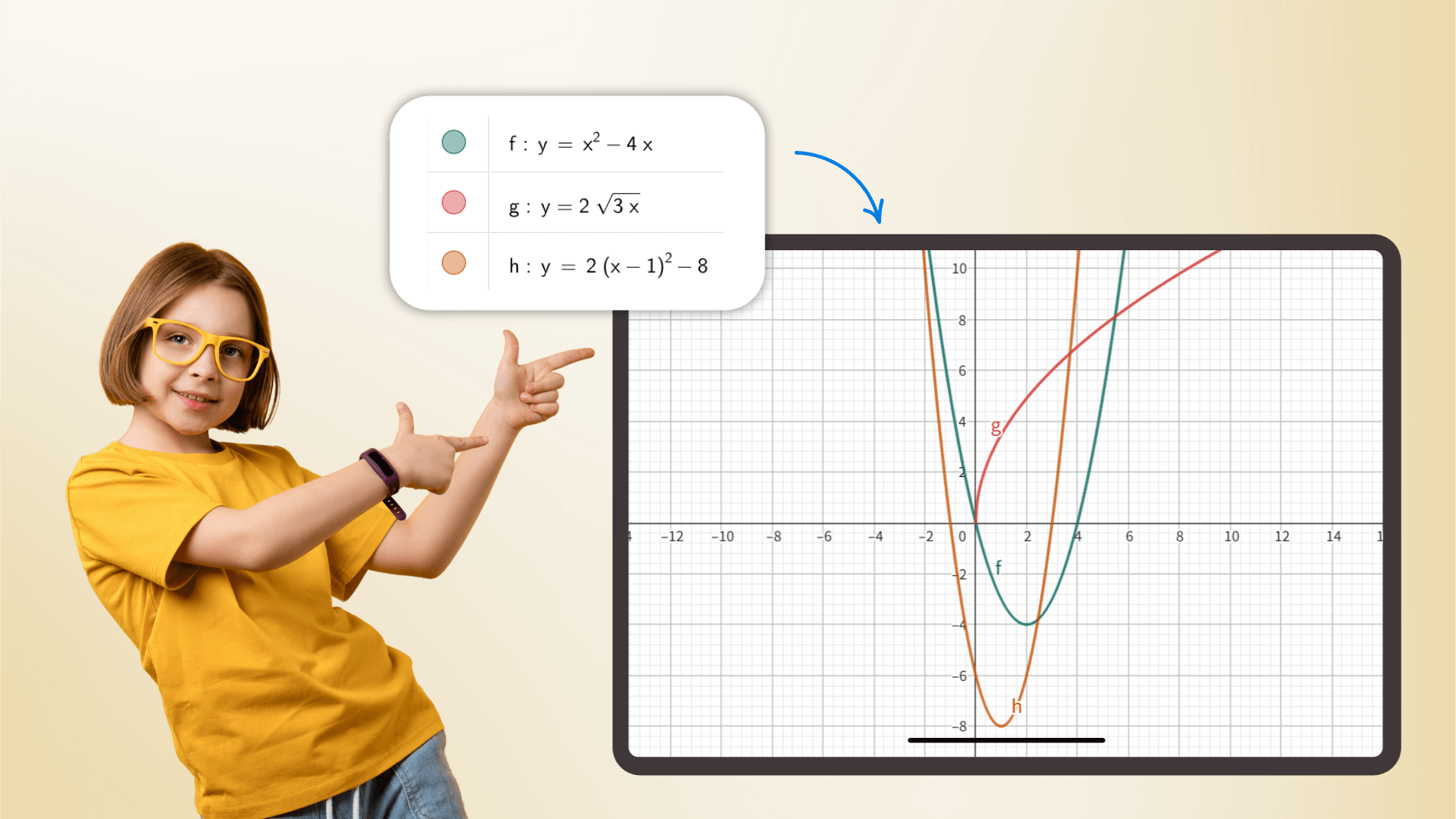
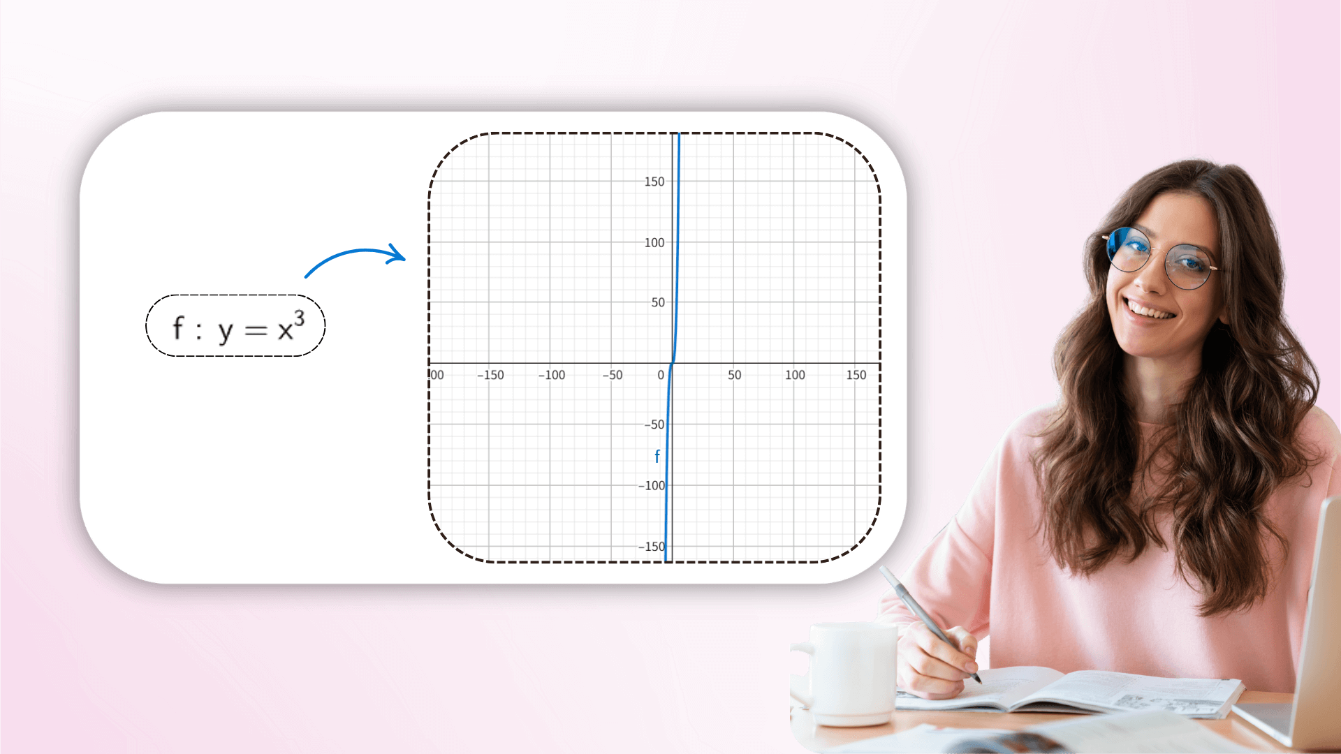
Graphing Calculator can plot various function graphs, including linear, parabolic, trigonometric, and logarithmic functions, and it can graph multiple equations at once in different colors. Just enter the function expression to quickly get an accurate graph and observe function trends and characteristics. The online graphing calculator helps everyone master math and avoid complex calculations.
As a scientific calculator, it handles everything from basic arithmetic to advanced mathematics, calculus, probability statistics and more. With precision driven calculations, it serves as an indispensable assistant for students and researchers alike, elevating efficiency across academic and professional contexts.
By adjusting parameter values in real time, users can observe the dynamic transformation of the image to understand how the coefficients affect the function geometry, from linear translation to complex transformations, linking abstract formulas with vision. This interactive exploration can deepen the understanding of mathematical equations.

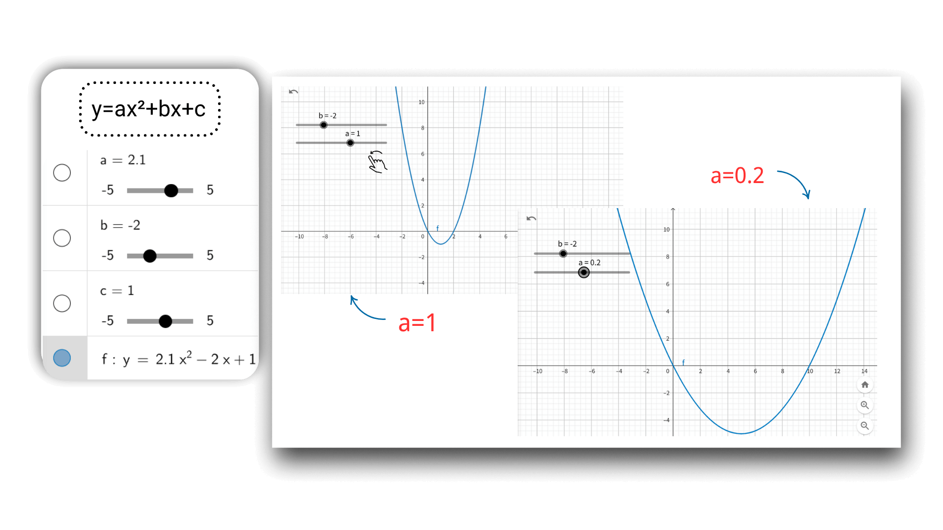
Using AI graphing technology, after entering the function, you can dynamically adjust the parameters through the slider, such as a, b, c of a quadratic function. The image will deform in real time like an animation, and the coordinate data will be updated synchronously, intuitively revealing the impact of parameter changes on the image, and better understanding the connection between mathematical concepts.
Adopting advanced calculation algorithms, we ensure that every calculation result has extremely high accuracy, providing reliable data support for your mathematical work. Simply input the array on our image calculator to generate various images with one click.
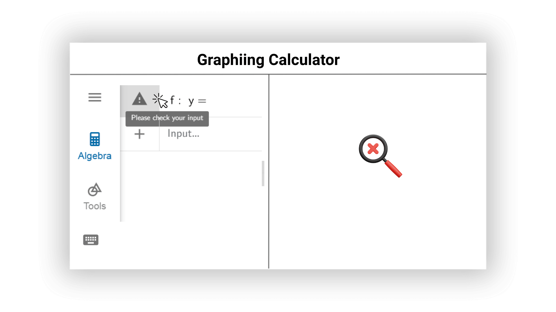
Our AI graphing calculator can check for possible errors in mathematical expressions online in real time and proactively give suggestions for modification. AI can promptly remind users of grammatical problems and unreasonable inputs to ensure accurate calculation results and high computational efficiency, and avoid errors in images and results.
1. ![]() Enter
Enter y = m x + b into the Input Bar and hit
the Enter key.
Hint: Graphing Calculator will
automatically create sliders for the parameters m and b when
pressing Enter. To show the sliders in the Graphics View,
select the disabled Visibility button in the Algebra View on
the left of the variables.
2. ![]() Create the intersection point A between the line and the
y-axis.
Create the intersection point A between the line and the
y-axis.
Hint: You may either use the Intersect
tool you can find in the Toolbox for points by selecting the
two objects, or use the command Intersect(f, yAxis).
3. ![]() Create a point B at the origin using the Intersect tool and
selecting the two axes.
Create a point B at the origin using the Intersect tool and
selecting the two axes.
4. ![]() Select the Segment tool from the Toolbox for lines and
create a segment between points A and B by selecting both
points.
Select the Segment tool from the Toolbox for lines and
create a segment between points A and B by selecting both
points.
Hint: Alternatively, you can use the
command Segment(A, B) as well.
5. ![]() Hide points A and B by clicking on the corresponding
enabled Visibility buttons on the left of their coordinates
in the Algebra View.
Hide points A and B by clicking on the corresponding
enabled Visibility buttons on the left of their coordinates
in the Algebra View.
6. ![]() Use the Slope tool from the Measure Toolbox to create the
slope (triangle) of the line by clicking on the line.
Use the Slope tool from the Measure Toolbox to create the
slope (triangle) of the line by clicking on the line.
7. ![]() Enhance the appearance of your construction using the Style
Bar (e.g., increase the line thickness of the segment to
make it visible on top of the y-axis).
Enhance the appearance of your construction using the Style
Bar (e.g., increase the line thickness of the segment to
make it visible on top of the y-axis).
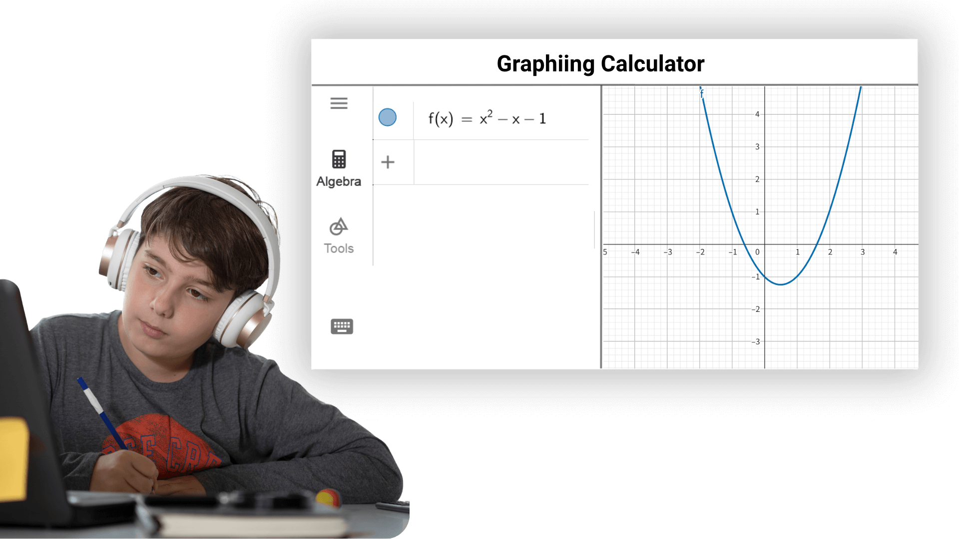
1. ![]() Type f(x) = x^2 into the Input Bar and hit the Enter
key.
Type f(x) = x^2 into the Input Bar and hit the Enter
key.
Which shape does the function graph have?
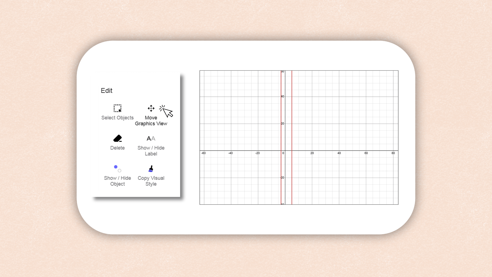
2. ![]() Use the Move tool and select the function. Click on the
Style Bar and select to unfix the function. You can now drag
the function in the Graphics View and watch how the equation
in the Algebra View adapts to your changes.
Use the Move tool and select the function. Click on the
Style Bar and select to unfix the function. You can now drag
the function in the Graphics View and watch how the equation
in the Algebra View adapts to your changes.
3. ![]() Change the function graph so that the corresponding
equation matches:
Change the function graph so that the corresponding
equation matches:
f(x) = (x + 2)²
f(x) = x² - 3
and
f(x) = (x - 4)² + 2.
4. ![]() Select the equation of the polynomial. Use the keyboard to
change the equation to f(x) = 3 x^2.
Select the equation of the polynomial. Use the keyboard to
change the equation to f(x) = 3 x^2.
How does
the function graph change?
5. ![]() Repeat changing the equation by typing in different values
for the parameter (e.g. 0.5, -2, -0.8, 3).
Repeat changing the equation by typing in different values
for the parameter (e.g. 0.5, -2, -0.8, 3).
1. ![]() Enter f(x) = a*x³ + b*x² + c*x + d into the Input
Bar and hit the Enter key.
Enter f(x) = a*x³ + b*x² + c*x + d into the Input
Bar and hit the Enter key.
Hint: Graphing Calculator will automatically
create sliders for the parameters a, b, c, and d.
2. ![]() Show the sliders in the Graphics View by selecting the
disabled Visibility buttons on the left of the corresponding
entries in the Algebra View.
Show the sliders in the Graphics View by selecting the
disabled Visibility buttons on the left of the corresponding
entries in the Algebra View.
3. ![]() Use the sliders in the Graphics View to change the values
of the parameters with the Move tool to
a = 0.2, b = -1.2, c = 0.6, d = 2.
Use the sliders in the Graphics View to change the values
of the parameters with the Move tool to
a = 0.2, b = -1.2, c = 0.6, d = 2.
4. ![]() Enter R = Root(f) into the Input Bar to display the
roots of the polynomial. The roots will be automatically
named R1, R2, and R3.
Enter R = Root(f) into the Input Bar to display the
roots of the polynomial. The roots will be automatically
named R1, R2, and R3.
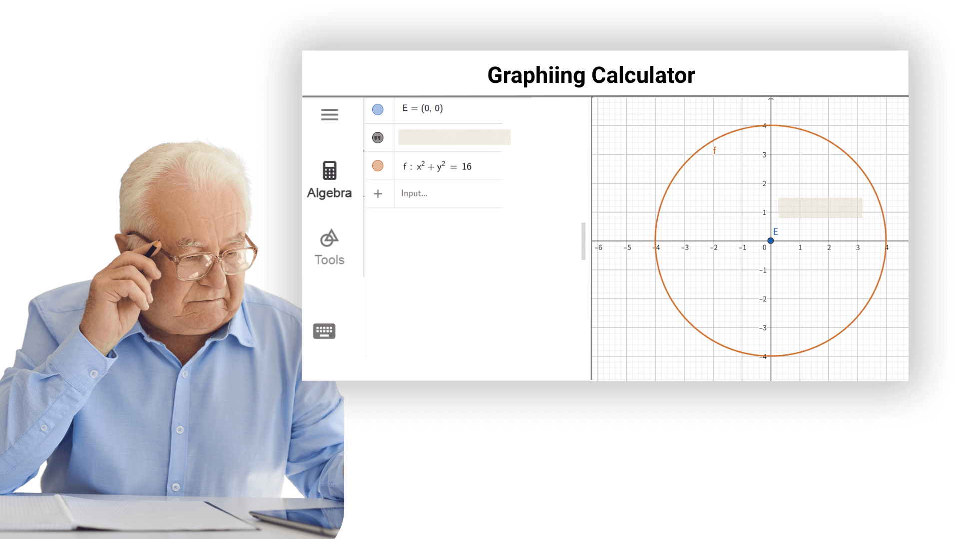
5. ![]() Enter E = Extremum(f) to display the local extrema
of the polynomial.
Enter E = Extremum(f) to display the local extrema
of the polynomial.
6. ![]() Use the Tangent tool to create the tangents to the
polynomial through the extrema E1 and E2.
Use the Tangent tool to create the tangents to the
polynomial through the extrema E1 and E2.
Hint: Open the Toolbox of Special Lines and
select the Tangent tool. Successively select point E1 and
the polynomial to create the tangent. Repeat for point
E2.
7. ![]() Systematically change the values of the sliders using the
Move tool to explore how the parameters affect the
polynomial.
Systematically change the values of the sliders using the
Move tool to explore how the parameters affect the
polynomial.
1. ![]() Enter the linear equation
line_1: y = m_1 x + b_1 into the Input Bar.
Enter the linear equation
line_1: y = m_1 x + b_1 into the Input Bar.
Hint: The input line_1 gives you line1.
2. ![]() Graphing Calculator will automatically create sliders for
the variables m_1 and b_1 when pressing
Enter.
Graphing Calculator will automatically create sliders for
the variables m_1 and b_1 when pressing
Enter.
3. ![]() Show the sliders in the Graphics View by clicking on the
disabled Visibility buttons next to their entry in the
Algebra View.
Show the sliders in the Graphics View by clicking on the
disabled Visibility buttons next to their entry in the
Algebra View.
4. ![]() Repeat steps 1 to 3 for the equation of
line_2: y = m_2 x + b_2.
Repeat steps 1 to 3 for the equation of
line_2: y = m_2 x + b_2.
5. ![]() Use the Style Bar to change the color of both lines and
their sliders.
Use the Style Bar to change the color of both lines and
their sliders.
6. ![]() Use the Text tool and create a dynamic text by entering
Line 1: in the appearing dialog and selecting
line_1 from the list of objects on the Objects tab of
the Advanced section.
Use the Text tool and create a dynamic text by entering
Line 1: in the appearing dialog and selecting
line_1 from the list of objects on the Objects tab of
the Advanced section.
7. ![]() Create a dynamic text with the static part
Line 2: and select line_2 from the list of
objects on the Objects tab of the Advanced section.
Create a dynamic text with the static part
Line 2: and select line_2 from the list of
objects on the Objects tab of the Advanced section.
8. ![]() Use the Style Bar to match the color of the texts with
their corresponding lines.
Use the Style Bar to match the color of the texts with
their corresponding lines.
9. ![]() Construct the intersection point A of both
line_1 and line_2 by either using the
Intersect tool, or by entering the command
Intersect(line_1, line_2) into the Input Bar.
Construct the intersection point A of both
line_1 and line_2 by either using the
Intersect tool, or by entering the command
Intersect(line_1, line_2) into the Input Bar.
10. ![]() Enter xcoordinate = x(A) into the Input Bar.
Enter xcoordinate = x(A) into the Input Bar.
Hint: x(A) gives you the x-coordinate of the
intersection point A.
11. ![]() Also, define ycoordinate = y(A).
Also, define ycoordinate = y(A).
Hint: y(A) gives you the y-coordinate of the
intersection point A.
12. ![]() Create a dynamic text with the static part
Solution: x = and select xcoordinate from the
list of objects on tab Objects.
Create a dynamic text with the static part
Solution: x = and select xcoordinate from the
list of objects on tab Objects.
13. ![]() Create a dynamic text with the static part y = and
select ycoordinate from the list of objects on tab
Objects.
Create a dynamic text with the static part y = and
select ycoordinate from the list of objects on tab
Objects.
14. ![]() Fix the texts so they can’t be moved accidentally by
selecting the texts and opening the Style Bar.
Fix the texts so they can’t be moved accidentally by
selecting the texts and opening the Style Bar.
1. ![]() Enter the polynomial f(x) = x^2/2 + 1 into the Input
Bar.
Enter the polynomial f(x) = x^2/2 + 1 into the Input
Bar.
2. ![]() Create a new point A on function f.
Create a new point A on function f.
Hint: Point A can only be moved along the
function.
3. ![]() Create tangent g to function f through point
A.
Create tangent g to function f through point
A.
4. ![]() Create the slope of tangent g using
m = Slope(g).
Create the slope of tangent g using
m = Slope(g).
5. ![]() Define point S = (x(A), m).
Define point S = (x(A), m).
Hint: x(A) gives you the x-coordinate of point
A.
6. ![]() Connect points A and S using a segment.
Connect points A and S using a segment.
7. ![]() Turn on the trace of point S and move point
A.
Turn on the trace of point S and move point
A.
Hint: Right-click point S (MacOS: Ctrl-click,
tablet: long tap) and select Show Trace.
1. ![]() Enter the function f(x) = sin(x) into the Input
Bar.
Enter the function f(x) = sin(x) into the Input
Bar.
2. ![]() Right-Click on the Graphics View and select Graphics... .
Select tab xAxis and change the unit to
Right-Click on the Graphics View and select Graphics... .
Select tab xAxis and change the unit to
π.
3. ![]() Create a new point A on function f.
Create a new point A on function f.
Hint: Point A can only be moved along the
function.
4. ![]() Create tangent g to function f through point
A.
Create tangent g to function f through point
A.
5. ![]() Create the slope of tangent g using the Slope
tool.
Create the slope of tangent g using the Slope
tool.
6. ![]() Define point S = (x(A), m).
Define point S = (x(A), m).
Hint: x(A) gives you the x-coordinate of point
A.
7. ![]() Connect points A and S using a segment.
Connect points A and S using a segment.
8. ![]() Turn on the trace of point S and move point
A.
Turn on the trace of point S and move point
A.
Hint: Right-click point S (MacOS: Ctrl-click,
tablet: long tap) and select Show Trace.
9. ![]() Right-click (MacOS: Ctrl-click, tablet: long tap) point
A and choose Animation from the context
menu.
Right-click (MacOS: Ctrl-click, tablet: long tap) point
A and choose Animation from the context
menu.
Hint: An Animation button appears in the lower
left corner of the Graphics View. It allows you to pause
or continue the animation.
1. ![]() Enter a x + b y ≤ c into the Input Bar and press
Enter.
Enter a x + b y ≤ c into the Input Bar and press
Enter.
Hint: You can use the Virtual Keyboard
to enter the ≤ symbol. Graphing Calculator will
automatically create sliders for the parameters a, b, and
c.
2. ![]() Use the Move tool to adjust the slider values so that a =
1, b = 1, and c = 3.
Use the Move tool to adjust the slider values so that a =
1, b = 1, and c = 3.
3. ![]() Change the increment of the sliders to 1.
Change the increment of the sliders to 1.
Hint:
Select number a and open the Style Bar of the Graphics View.
Open the settings of number a and select the Slider tab.
Set the increment to 1 and repeat for numbers b and c.
4. ![]() Drag the background of the Graphics View to move the origin
to the center.
Drag the background of the Graphics View to move the origin
to the center.
5. ![]() Zoom out to make a bigger part of the coordinate system
visible on screen.
Zoom out to make a bigger part of the coordinate system
visible on screen.
6. ![]() Set the distance between the marks on the axes to 1.
Set the distance between the marks on the axes to 1.
Hint:
Make sure that no object is selected before you open the
Style Bar of the Graphics View.
Open the settings of the axes.
Select the xAxis tab and set the distance to 1.
Repeat on the yAxis tab.
1. ![]() Enter
Sequence(Segment((a, 0), (0, a)), a, 1, 10, 0.5) into
the Input Bar and press Enter.
Enter
Sequence(Segment((a, 0), (0, a)), a, 1, 10, 0.5) into
the Input Bar and press Enter.
2. ![]() Create a slider s for a number with interval from 1
to 10 and increment 1.
Create a slider s for a number with interval from 1
to 10 and increment 1.
3. ![]() Enter Sequence((i, i), i, 0, s) into the Input Bar
and press Enter.
Enter Sequence((i, i), i, 0, s) into the Input Bar
and press Enter.
4. ![]() Move the slider s to check the construction.
Move the slider s to check the construction.
1. ![]() Open the Settings of the Graphics View using the Style
Bar.
Open the Settings of the Graphics View using the Style
Bar.
2. ![]() On tab xAxis set the distance of tick marks to 1 by
checking the box Distance and entering 1 into the text
field.
On tab xAxis set the distance of tick marks to 1 by
checking the box Distance and entering 1 into the text
field.
3. ![]() On tab Basic set the minimum of the xAxis to -11 and the
maximum to 11.
On tab Basic set the minimum of the xAxis to -11 and the
maximum to 11.
4. ![]() On tab yAxis uncheck Show yAxis and close the
Settings.
On tab yAxis uncheck Show yAxis and close the
Settings.
5. ![]() Create two sliders a and b, both with
Interval -5 to 5 and Increment 1.
Create two sliders a and b, both with
Interval -5 to 5 and Increment 1.
6. ![]() Show the value of the sliders instead of their names using
the Style Bar.
Show the value of the sliders instead of their names using
the Style Bar.
7. ![]() Create points A = (0, 1) and
B = A + (a, 0).
Create points A = (0, 1) and
B = A + (a, 0).
Hint: The distance of point B to point A is
determined by slider a.
8. ![]() Create a vector u = Vector(A, B) which has the
length a.
Create a vector u = Vector(A, B) which has the
length a.
9. ![]() Create points C = B + (0, 1) and
D = C + (b, 0).
Create points C = B + (0, 1) and
D = C + (b, 0).
10. ![]() Create vector v = Vector(C, D) which has the length
b.
Create vector v = Vector(C, D) which has the length
b.
11. ![]() Create point R = (x(D), 0).
Create point R = (x(D), 0).
Hint: The input x(D) gives you the x-coordinate
of point D. Thus, point R shows the result of the addition
on the number line.
12. ![]() Create point Z = (0, 0).
Create point Z = (0, 0).
13. ![]() Create three segments c = Segment(Z, A),
d = Segment(B, C), and
e = Segment(D, R).
Create three segments c = Segment(Z, A),
d = Segment(B, C), and
e = Segment(D, R).
14. ![]() Use the Style Bar to enhance your construction (e.g. match
the color of sliders and vectors, change line style, fix
sliders, hide labels and points).
Use the Style Bar to enhance your construction (e.g. match
the color of sliders and vectors, change line style, fix
sliders, hide labels and points).
1. ![]() Create a horizontal slider named Columns for a
number with interval from 1 to 10, increment 1, and width
300.
Create a horizontal slider named Columns for a
number with interval from 1 to 10, increment 1, and width
300.
Hint: You can change the width of the
slider in the Settings tab under Slider.
2. ![]() Create a new point A.
Create a new point A.
3. ![]() Construct segment f with the given length
Columns starting from point A.
Construct segment f with the given length
Columns starting from point A.
4. ![]() Move the Columns slider to observe the segment with the
specified length.
Move the Columns slider to observe the segment with the
specified length.
5. ![]() Construct a perpendicular line g to segment f
through point A.
Construct a perpendicular line g to segment f
through point A.
6. ![]() Construct a perpendicular line h to segment f
through point B.
Construct a perpendicular line h to segment f
through point B.
7. ![]() Create a vertical slider named Rows for a number
with interval from 1 to 10, increment 1, and width 300.
Create a vertical slider named Rows for a number
with interval from 1 to 10, increment 1, and width 300.
Hint:
You can select the orientation of the slider in the Slider
dialog under the Slider tab.
8. ![]() Create a circle c with center A and radius
Rows.
Create a circle c with center A and radius
Rows.
9. ![]() Move the Rows slider to observe the circle with the
specified radius.
Move the Rows slider to observe the circle with the
specified radius.
10. ![]() Intersect circle c with line g to get intersection point
C.
Intersect circle c with line g to get intersection point
C.
Hint: When selecting the Intersect
tool click on the intersection point above point A to only
create this point.
11. ![]() Create a parallel line i to segment f through
intersection point C.
Create a parallel line i to segment f through
intersection point C.
12. ![]() Intersect lines i and h to get intersection point
D.
Intersect lines i and h to get intersection point
D.
13. ![]() Construct a polygon ABDC.
Construct a polygon ABDC.
14. ![]() Hide all lines, circle c, and segment f.
Hide all lines, circle c, and segment f.
15. ![]() Hide labels of segments using the Style Bar.
Hide labels of segments using the Style Bar.
16. ![]() Set both sliders Columns and Rows to value 10.
Set both sliders Columns and Rows to value 10.
17. ![]() Create a list of vertical segments using:
Create a list of vertical segments using: Sequence(Segment(A + i*(1, 0), C + i*(1, 0)), i, 1,
Columns)
Note: A + i*(1, 0) specifies a series of points starting at
point A with distance 1 from each other.
C + i*(1, 0)
specifies a series of points starting at point C with
distance 1 from each other.
Segment(A + i*(1, 0), C +
i*(1, 0))creates a list of segments between pairs of these
points. Note, that the endpoints of the segments are not
shown in the Graphics View.
Slider Column determines
the number of segments created.
18. ![]() Create a list of horizontal segments.
Create a list of horizontal segments.Sequence(Segment(A + i*(0, 1), B + i*(0, 1)), i, 1,
Rows)
19. ![]() Move the Columns and Rows sliders to observe the
construction.
Move the Columns and Rows sliders to observe the
construction.
20. ![]() Insert static and dynamic text to state the multiplication
problem using the values of Columns and Rows as the
factors:
Insert static and dynamic text to state the multiplication
problem using the values of Columns and Rows as the
factors:text1: Columnstext2: *text3: Rowstext4: =
21. ![]() Calculate the result of the multiplication:
Calculate the result of the multiplication:
result = Columns * Rows
22. ![]() Insert dynamic text5:
Insert dynamic text5: result
23. ![]() Hide points A, B, C, and D.
Hide points A, B, C, and D.
24. ![]() Enhance your construction using the Style Bar.
Enhance your construction using the Style Bar.
AI graphing calculator is a powerful assistant for students to learn mathematics. From middle school to university, It is algebra, geometry, calculus or statistics courses that can help students better understand and master mathematical knowledge and improve learning efficiency and grades. Teachers can use it to conduct teaching demonstrations and create vivid teaching courseware to stimulate students' interest and enthusiasm in learning.
It provides researchers with powerful mathematical tools to facilitate data processing, experimental analysis, model building, and theoretical verification. In various scientific fields such as physics, chemistry, biology, and engineering, graphic calculators can be used to quickly and accurately complete complex mathematical operations and data analysis, assisting the smooth development of scientific research.
Use the graphing calculator to draw supply and demand curves, compound growth models, etc, analyze the intersection of marginal cost and revenue functions, and assist in business decision-making.
Graphing Calculator benefits students from elementary to university levels. It helps them grasp math concepts and cultivates problem solving skills.

Math teachers can use graph calculator to create lesson materials and demonstrate concepts and problem - solving processes, enhancing teaching effectiveness and interaction.

Researchers in various fields rely on it for complex math calculations and data analysis. Graphing calculator online precise results accelerate research.

Say goodbye to tedious manual drawing, generate professional data visualization charts with one click, draw function graphs online, annotate mean and variance in real time, dynamically fit regression curves, and efficiently complete data integration and analysis.

Graphing calculators help software engineers visualize filter algorithms and optimize rendering parameters, ensuring pixel-perfect function performance.

For architectural designers, graphing calculators are parametric design powerhouses, input curve equations to generate function/displacement graphs, visually validate structural mechanics, and slash design cycles.

All functions do not require registration or payment, and you can use them all the time.
Maintain high precision when calculating advanced problems such as matrix determinants and integrals to avoid scientific research errors.
The calculation is completed entirely in the browser, no data is uploaded, and the page is cleared when it is closed.
No need to download and install, mobile phones and computers can be used immediately.
Focus on the essence of learning, no pop-ups, no ads, and improve concentration.
Whether it is academic, scientific research, office or engineering applications, we can meet your graphical computing needs.
You don't need to register or download any software. Just enter our website in your browser and start using this powerful graphing calculator tool. You can experience its convenience instantly.
Yes, our AI graphing calculator is completely free. Despite being free, it doesn't restrict any core features. You can fully utilize its graphing, calculation, and data analysis functions without any cost. We aim to provide a convenient and efficient math tool for everyone.
We prioritize your data security and privacy. All your calculations, graphs, and input data are processed locally in your browser and are never uploaded or stored on our servers. You can use it with confidence, knowing your data is safe.
To input a function, simply type the formula into the input box on the homepage. For example, enter "y=2x^2" or "f(x)=sin(x)". The calculator will automatically process your input and display the graph.
Yes, the AI Graphing Calculator can handle a variety of functions, from simple linear equations to advanced ones like integrals, derivatives, and multivariable equations. It's suitable for both basic and advanced mathematical needs, making it ideal for students and professionals.
Yes, it is fully accessible on mobile devices. You can use it on smartphones or tablets, and it's optimized for all screen sizes, ensuring a seamless experience wherever you are.